3. The Classical Runge–Kutta Method (RK4)

Author

Miraj Samarakkody

Published

October 26, 2026

RK4 uses four slopes per step and has order 4. For smooth, non-stiff problems it gives an excellent balance of accuracy and simplicity, which is why it is the method most people mean by “Runge–Kutta”. This section derives it, introduces the Butcher tableau notation that describes every Runge–Kutta method, and explains the order conditions that determine a method’s order.

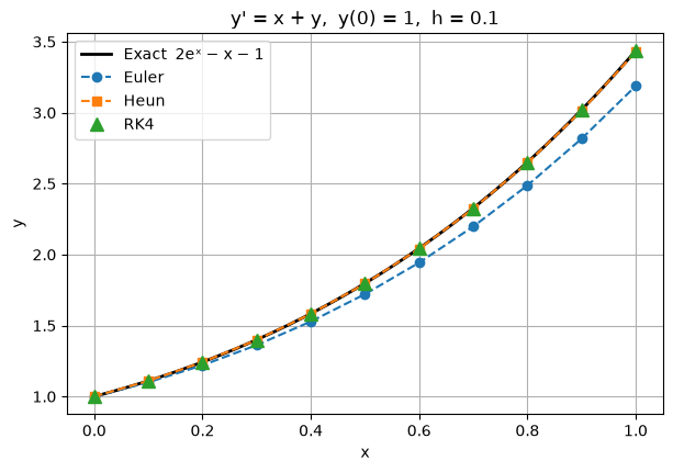
Test problem: \(y' = x + y\), \(y(0) = 1\), exact solution \(y = 2e^{x} - x - 1\).

Quick note: RK4 with a calculator

Use: solve \(y' = f(x, y)\), \(y(x_0) = y_0\), one step at a time with step size \(h\).

One step (four slopes):

  1. Slope at the start: \(k_1 = f(x_n,\ y_n)\)
  2. Slope at the middle, using \(k_1\): \(k_2 = f\!\left(x_n + \tfrac{h}{2},\ y_n + \tfrac{h}{2}k_1\right)\)
  3. Slope at the middle again, using \(k_2\): \(k_3 = f\!\left(x_n + \tfrac{h}{2},\ y_n + \tfrac{h}{2}k_2\right)\)
  4. Slope at the end, using \(k_3\): \(k_4 = f(x_n + h,\ y_n + h\,k_3)\)
  5. Weighted average and step: \(y_{n+1} = y_n + \dfrac{h}{6}(k_1 + 2k_2 + 2k_3 + k_4)\)
  6. Move along: \(x_{n+1} = x_n + h\), then repeat.

Each step needs only multiplication, addition and \(f\), so a basic calculator is enough.

Example: \(y' = x + y\), \(y(0) = 1\), \(h = 0.1\). Find \(y(0.2)\). Here \(h/2 = 0.05\) and \(h/6 = 0.0166667\).

Step 1 (\(x_0 = 0\), \(y_0 = 1\))

  • \(k_1 = 0 + 1 = 1\)
  • \(k_2 = 0.05 + (1 + 0.05 \times 1) = 0.05 + 1.05 = 1.1\)
  • \(k_3 = 0.05 + (1 + 0.05 \times 1.1) = 0.05 + 1.055 = 1.105\)
  • \(k_4 = 0.1 + (1 + 0.1 \times 1.105) = 0.1 + 1.1105 = 1.2105\)
  • \(k_1 + 2k_2 + 2k_3 + k_4 = 1 + 2.2 + 2.21 + 1.2105 = 6.6205\)
  • \(y_1 = 1 + \tfrac{0.1}{6}(6.6205) = \mathbf{1.1103417}\)

Step 2 (\(x_1 = 0.1\), \(y_1 = 1.1103417\))

  • \(k_1 = 0.1 + 1.1103417 = 1.2103417\)
  • \(k_2 = 0.15 + (1.1103417 + 0.05 \times 1.2103417) = 0.15 + 1.1708588 = 1.3208588\)
  • \(k_3 = 0.15 + (1.1103417 + 0.05 \times 1.3208588) = 0.15 + 1.1763846 = 1.3263846\)
  • \(k_4 = 0.2 + (1.1103417 + 0.1 \times 1.3263846) = 0.2 + 1.2429802 = 1.4429802\)
  • \(k_1 + 2k_2 + 2k_3 + k_4 = 1.2103417 + 2.6417176 + 2.6527692 + 1.4429802 = 7.9478087\)
  • \(y_2 = 1.1103417 + \tfrac{0.1}{6}(7.9478087) = \mathbf{1.2428052}\)

Check: the exact answer is \(y(0.2) = 2e^{0.2} - 1.2 = 1.2428055\), so the error is about \(3 \times 10^{-7}\). Heun (RK2) with the same \(h\) has an error of about \(0.0008\), roughly 2000 times larger.

Tips for working by hand

  • Lay it out as a table: \(n\), \(x_n\), \(y_n\), \(k_1\), \(k_2\), \(k_3\), \(k_4\), \(y_{n+1}\).
  • \(k_2\) and \(k_3\) both use \(x_n + h/2\). Only the \(y\) value changes.
  • Don’t forget the 2s: the middle slopes count twice.
  • Keep 6 to 7 decimal places in the middle of the working, because RK4 is accurate enough that rounding errors start to show.
  • Halving \(h\) cuts the error to about \(\tfrac{1}{16}\).
Code
import numpy as np
import matplotlib.pyplot as plt

plt.rcParams["figure.figsize"] = (7, 4.5)
plt.rcParams["axes.grid"] = True
np.set_printoptions(precision=6, suppress=True)

f = lambda x, y: x + y
exact = lambda x: 2 * np.exp(x) - x - 1

def euler(f, x0, y0, h, n):
    x, y = np.zeros(n + 1), np.zeros(n + 1)
    x[0], y[0] = x0, y0
    for i in range(n):
        y[i + 1] = y[i] + h * f(x[i], y[i])
        x[i + 1] = x[i] + h
    return x, y

def heun(f, x0, y0, h, n):
    x, y = np.zeros(n + 1), np.zeros(n + 1)
    x[0], y[0] = x0, y0
    for i in range(n):
        k1 = f(x[i], y[i])
        k2 = f(x[i] + h, y[i] + h * k1)
        y[i + 1] = y[i] + h / 2 * (k1 + k2)
        x[i + 1] = x[i] + h
    return x, y

3.1 Derivation from Simpson’s rule

Simpson’s rule weights the midpoint four times as heavily as the ends:

\[\int_{x_n}^{x_{n+1}} f\,dx \approx \frac{h}{6}\Big[f_{\text{start}} + 4 f_{\text{mid}} + f_{\text{end}}\Big].\]

RK4 estimates the midpoint slope twice, each time more accurately than the last, and splits the weight \(4\) into \(2 + 2\):

\[ \begin{aligned} k_1 &= f(x_n,\ y_n) && \text{slope at the start}\\ k_2 &= f\!\left(x_n + \tfrac{h}{2},\ y_n + \tfrac{h}{2}k_1\right) && \text{slope at the midpoint, reached using } k_1\\ k_3 &= f\!\left(x_n + \tfrac{h}{2},\ y_n + \tfrac{h}{2}k_2\right) && \text{slope at the midpoint, reached using the better } k_2\\ k_4 &= f\!\left(x_n + h,\ y_n + h k_3\right) && \text{slope at the end, reached using } k_3\\[4pt] y_{n+1} &= y_n + \tfrac{h}{6}\big(k_1 + 2k_2 + 2k_3 + k_4\big) \end{aligned} \]

The weights \(\tfrac{1}{6}, \tfrac{2}{6}, \tfrac{2}{6}, \tfrac{1}{6}\) add up to 1, so \(\tfrac{1}{6}(k_1 + 2k_2 + 2k_3 + k_4)\) is a weighted average slope. The local error is \(O(h^5)\) and the global error \(O(h^4)\): RK4 is order 4, and halving \(h\) divides the error by about 16. Each step costs 4 evaluations of \(f\).

When \(f\) depends on \(x\) only, \(y' = f(x)\), the stages \(k_2\) and \(k_3\) coincide and RK4 is Simpson’s rule.

Code
def rk4(f, x0, y0, h, n):
    x, y = np.zeros(n + 1), np.zeros(n + 1)
    x[0], y[0] = x0, y0
    for i in range(n):
        k1 = f(x[i], y[i])
        k2 = f(x[i] + h / 2, y[i] + h / 2 * k1)
        k3 = f(x[i] + h / 2, y[i] + h / 2 * k2)
        k4 = f(x[i] + h, y[i] + h * k3)
        y[i + 1] = y[i] + h / 6 * (k1 + 2 * k2 + 2 * k3 + k4)
        x[i + 1] = x[i] + h
    return x, y

Worked example: RK4 by hand, first step with \(h = 0.1\)

stage evaluation point \((x, y)\) slope
\(k_1\) \((0,\ 1)\) \(1\)
\(k_2\) \((0.05,\ 1 + 0.05 \cdot 1) = (0.05,\ 1.05)\) \(1.1\)
\(k_3\) \((0.05,\ 1 + 0.05 \cdot 1.1) = (0.05,\ 1.055)\) \(1.105\)
\(k_4\) \((0.1,\ 1 + 0.1 \cdot 1.105) = (0.1,\ 1.1105)\) \(1.2105\)

\[y_1 = 1 + \frac{0.1}{6}\big(1 + 2(1.1) + 2(1.105) + 1.2105\big) = 1 + \frac{0.1}{6}(6.6205) = 1.1103417.\]

Exact: \(y(0.1) = 1.1103418\). The error is \(1.7 \times 10^{-7}\), about 60,000 times smaller than Euler’s first step.

3.2 Seeing the slopes

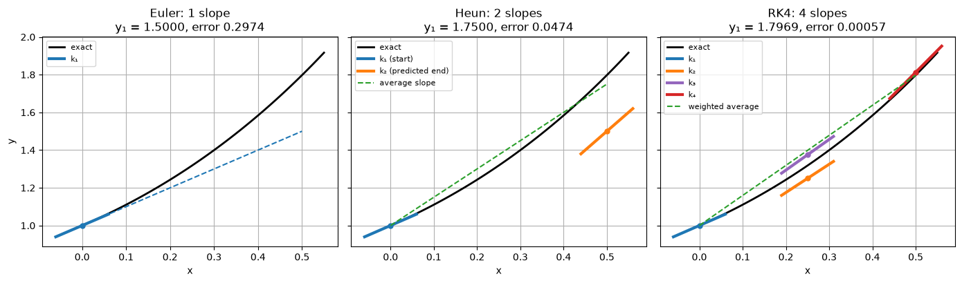
One large step (\(h = 0.5\)) from \((0, 1)\) shows where each method samples the slope. Short arrows mark each sampled slope; the dashed line is the step actually taken.

Code
h, x0, y0 = 0.5, 0.0, 1.0
xf = np.linspace(0, 0.55, 100)

def slope_mark(ax, x, y, s, color, label=None):
    d = 0.06
    ax.plot([x - d, x + d], [y - d * s, y + d * s], color=color, lw=3, label=label)
    ax.plot(x, y, "o", color=color, ms=5)

fig, axes = plt.subplots(1, 3, figsize=(14, 4.2), sharey=True)
for ax in axes:
    ax.plot(xf, exact(xf), "k", lw=2, label="exact")
    ax.set_xlabel("x")
axes[0].set_ylabel("y")

# Euler
k1 = f(x0, y0)
y_e = y0 + h * k1
slope_mark(axes[0], x0, y0, k1, "C0", "k₁")
axes[0].plot([x0, h], [y0, y_e], "C0--")
axes[0].set_title(f"Euler: 1 slope\ny₁ = {y_e:.4f}, error {exact(h) - y_e:.4f}")

# Heun
k2 = f(x0 + h, y0 + h * k1)
y_h = y0 + h / 2 * (k1 + k2)
slope_mark(axes[1], x0, y0, k1, "C0", "k₁ (start)")
slope_mark(axes[1], x0 + h, y0 + h * k1, k2, "C1", "k₂ (predicted end)")
axes[1].plot([x0, h], [y0, y_h], "C2--", label="average slope")
axes[1].set_title(f"Heun: 2 slopes\ny₁ = {y_h:.4f}, error {exact(h) - y_h:.4f}")

# RK4
r1 = f(x0, y0)
r2 = f(x0 + h / 2, y0 + h / 2 * r1)
r3 = f(x0 + h / 2, y0 + h / 2 * r2)
r4 = f(x0 + h, y0 + h * r3)
y_r = y0 + h / 6 * (r1 + 2 * r2 + 2 * r3 + r4)
slope_mark(axes[2], x0, y0, r1, "C0", "k₁")
slope_mark(axes[2], x0 + h / 2, y0 + h / 2 * r1, r2, "C1", "k₂")
slope_mark(axes[2], x0 + h / 2, y0 + h / 2 * r2, r3, "C4", "k₃")
slope_mark(axes[2], x0 + h, y0 + h * r3, r4, "C3", "k₄")
axes[2].plot([x0, h], [y0, y_r], "C2--", label="weighted average")
axes[2].set_title(f"RK4: 4 slopes\ny₁ = {y_r:.4f}, error {exact(h) - y_r:.5f}")

for ax in axes:
    ax.legend(loc="upper left", fontsize=8)
plt.tight_layout()
print(f"exact y(0.5) = {exact(h):.6f}")
exact y(0.5) = 1.797443

3.3 Why the order is what it is: matching the Taylor series

For the test problem, the exact solution after one step from \((0, 1)\) has the Taylor series

\[y(h) = 2e^{h} - h - 1 = 1 + h + h^2 + \frac{h^3}{3} + \frac{h^4}{12} + \frac{h^5}{60} + \cdots\]

Expanding each method’s formula for one step, symbolically in \(h\):

Method One step gives First term missed (local error) Predicted at \(h=0.1\) Actual
Euler \(1 + h\) \(h^2\) \(1.0 \times 10^{-2}\) \(1.03 \times 10^{-2}\)
Heun \(1 + h + h^2\) \(h^3/3\) \(3.3 \times 10^{-4}\) \(3.42 \times 10^{-4}\)
RK4 \(1 + h + h^2 + \frac{h^3}{3} + \frac{h^4}{12}\) \(h^5/60\) \(1.7 \times 10^{-7}\) \(1.69 \times 10^{-7}\)

(For RK4: \(k_1 = 1\), \(k_2 = 1 + h\), \(k_3 = 1 + h + \tfrac{h^2}{2}\), \(k_4 = 1 + 2h + h^2 + \tfrac{h^3}{2}\); substituting gives the expression in the table.)

This is the real meaning of order: a method of order \(p\) reproduces the Taylor series of the true solution through the \(h^p\) term. The first term it misses, of size \(h^{p+1}\), is the local error. Over \(1/h\) steps these add up to a global error of \(h^p\).

3.4 All three methods side by side

Code
h, n = 0.1, 10
x, ye = euler(f, 0, 1, h, n)
_, yh = heun(f, 0, 1, h, n)
_, yr = rk4(f, 0, 1, h, n)
yx = exact(x)

print(f"{'x':>5} {'Euler':>10} {'Heun':>10} {'RK4':>12} {'Exact':>12} "
      f"{'|err| Eul':>10} {'|err| Heun':>10} {'|err| RK4':>10}")
for i in range(n + 1):
    print(f"{x[i]:5.1f} {ye[i]:10.6f} {yh[i]:10.6f} {yr[i]:12.8f} {yx[i]:12.8f} "
          f"{abs(ye[i]-yx[i]):10.2e} {abs(yh[i]-yx[i]):10.2e} {abs(yr[i]-yx[i]):10.2e}")

xf = np.linspace(0, 1, 200)
plt.plot(xf, exact(xf), "k", lw=2, label="Exact  2eˣ − x − 1")
plt.plot(x, ye, "o--", label="Euler")
plt.plot(x, yh, "s--", label="Heun")
plt.plot(x, yr, "^", ms=8, label="RK4")
plt.title("y' = x + y,  y(0) = 1,  h = 0.1")
plt.xlabel("x"); plt.ylabel("y"); plt.legend();
    x      Euler       Heun          RK4        Exact  |err| Eul |err| Heun  |err| RK4
  0.0   1.000000   1.000000   1.00000000   1.00000000   0.00e+00   0.00e+00   0.00e+00
  0.1   1.100000   1.110000   1.11034167   1.11034184   1.03e-02   3.42e-04   1.69e-07
  0.2   1.220000   1.242050   1.24280514   1.24280552   2.28e-02   7.56e-04   3.75e-07
  0.3   1.362000   1.398465   1.39971699   1.39971762   3.77e-02   1.25e-03   6.21e-07
  0.4   1.528200   1.581804   1.58364848   1.58364940   5.54e-02   1.85e-03   9.15e-07
  0.5   1.721020   1.794894   1.79744128   1.79744254   7.64e-02   2.55e-03   1.26e-06
  0.6   1.943122   2.040857   2.04423592   2.04423760   1.01e-01   3.38e-03   1.68e-06
  0.7   2.197434   2.323147   2.32750325   2.32750541   1.30e-01   4.36e-03   2.16e-06
  0.8   2.487178   2.645578   2.65107913   2.65108186   1.64e-01   5.50e-03   2.73e-06
  0.9   2.815895   3.012364   3.01920283   3.01920622   2.03e-01   6.84e-03   3.39e-06
  1.0   3.187485   3.428162   3.43655949   3.43656366   2.49e-01   8.40e-03   4.17e-06

3.5 Butcher tableaux

Every explicit Runge–Kutta method with \(s\) stages has the form

\[ \begin{aligned} k_i &= f\Big(x_n + c_i h,\ \ y_n + h\sum_{j=1}^{i-1} a_{ij}\,k_j\Big), \qquad i = 1, \dots, s,\\ y_{n+1} &= y_n + h \sum_{i=1}^{s} b_i\,k_i, \end{aligned} \]

and is completely described by the numbers \(c_i\), \(a_{ij}\) and \(b_i\). They are written in a Butcher tableau:

\[ \begin{array}{c|cccc} c_1 & & & & \\ c_2 & a_{21} & & & \\ \vdots & \vdots & \ddots & & \\ c_s & a_{s1} & \cdots & a_{s,s-1} & \\ \hline & b_1 & \cdots & b_{s-1} & b_s \end{array} \]

  • “Explicit” means the matrix \(A = (a_{ij})\) is strictly lower triangular: stage \(i\) uses only stages before it.
  • Almost all methods satisfy \(c_i = \sum_j a_{ij}\): each stage is evaluated at the \(x\) value that its \(y\) value corresponds to.
  • The \(b_i\) are the weights of the final average; they add up to 1.

\[ \underset{\text{Euler}}{\begin{array}{c|c} 0 & \\ \hline & 1 \end{array}} \qquad \underset{\text{Heun}}{\begin{array}{c|cc} 0 & & \\ 1 & 1 & \\ \hline & \tfrac12 & \tfrac12 \end{array}} \qquad \underset{\text{Midpoint}}{\begin{array}{c|cc} 0 & & \\ \tfrac12 & \tfrac12 & \\ \hline & 0 & 1 \end{array}} \qquad \underset{\text{Kutta's 3rd order}}{\begin{array}{c|ccc} 0 & & & \\ \tfrac12 & \tfrac12 & & \\ 1 & -1 & 2 & \\ \hline & \tfrac16 & \tfrac23 & \tfrac16 \end{array}} \]

\[ \underset{\text{Classical RK4}}{\begin{array}{c|cccc} 0 & & & & \\ \tfrac12 & \tfrac12 & & & \\ \tfrac12 & 0 & \tfrac12 & & \\ 1 & 0 & 0 & 1 & \\ \hline & \tfrac16 & \tfrac13 & \tfrac13 & \tfrac16 \end{array}} \qquad \underset{\text{3/8 rule}}{\begin{array}{c|cccc} 0 & & & & \\ \tfrac13 & \tfrac13 & & & \\ \tfrac23 & -\tfrac13 & 1 & & \\ 1 & 1 & -1 & 1 & \\ \hline & \tfrac18 & \tfrac38 & \tfrac38 & \tfrac18 \end{array}} \]

One function can now run any explicit Runge–Kutta method, given its tableau.

Code
TABLEAUX = {
    "Euler":   dict(c=[0], A=[[0]], b=[1]),
    "Heun":    dict(c=[0, 1], A=[[0, 0], [1, 0]], b=[1/2, 1/2]),
    "Midpoint": dict(c=[0, 1/2], A=[[0, 0], [1/2, 0]], b=[0, 1]),
    "Ralston": dict(c=[0, 2/3], A=[[0, 0], [2/3, 0]], b=[1/4, 3/4]),
    "Kutta3":  dict(c=[0, 1/2, 1], A=[[0, 0, 0], [1/2, 0, 0], [-1, 2, 0]], b=[1/6, 2/3, 1/6]),
    "RK4":     dict(c=[0, 1/2, 1/2, 1],
                    A=[[0, 0, 0, 0], [1/2, 0, 0, 0], [0, 1/2, 0, 0], [0, 0, 1, 0]],
                    b=[1/6, 1/3, 1/3, 1/6]),
    "3/8 rule": dict(c=[0, 1/3, 2/3, 1],
                     A=[[0, 0, 0, 0], [1/3, 0, 0, 0], [-1/3, 1, 0, 0], [1, -1, 1, 0]],
                     b=[1/8, 3/8, 3/8, 1/8]),
}
TABLEAUX = {name: {k: np.array(v, dtype=float) for k, v in t.items()} for name, t in TABLEAUX.items()}


def explicit_rk(tableau, f, x0, y0, h, n):
    A, b, c = tableau["A"], tableau["b"], tableau["c"]
    s = len(b)
    x, y = np.zeros(n + 1), np.zeros(n + 1)
    x[0], y[0] = x0, y0
    for i in range(n):
        k = np.zeros(s)
        for j in range(s):
            k[j] = f(x[i] + c[j] * h, y[i] + h * (A[j, :j] @ k[:j]))
        y[i + 1] = y[i] + h * (b @ k)
        x[i + 1] = x[i] + h
    return x, y


print("max difference between explicit_rk(RK4) and rk4:",
      np.max(np.abs(explicit_rk(TABLEAUX["RK4"], f, 0, 1, 0.1, 10)[1] - rk4(f, 0, 1, 0.1, 10)[1])))
max difference between explicit_rk(RK4) and rk4: 8.881784197001252e-16

3.6 Order conditions

Section 2.3 found the conditions for order 2 by matching Taylor series. Doing the same at higher order gives one condition for each distinct term (“elementary differential”) in the Taylor series of the exact solution. In tableau notation, with \(\mathbf{c} = (c_i)\), \(\mathbf{1} = (1, \dots, 1)\) and powers of vectors taken componentwise:

Order New conditions
1 \(\mathbf{b}\cdot\mathbf{1} = 1\)
2 \(\mathbf{b}\cdot\mathbf{c} = \tfrac12\)
3 \(\mathbf{b}\cdot\mathbf{c}^2 = \tfrac13\), \(\quad \mathbf{b}\cdot A\mathbf{c} = \tfrac16\)
4 \(\mathbf{b}\cdot\mathbf{c}^3 = \tfrac14\), \(\quad \mathbf{b}\cdot(\mathbf{c} \ast A\mathbf{c}) = \tfrac18\), \(\quad \mathbf{b}\cdot A\mathbf{c}^2 = \tfrac1{12}\), \(\quad \mathbf{b}\cdot A^2\mathbf{c} = \tfrac1{24}\)

(Here \(\ast\) is the componentwise product.) A method has order \(p\) if it satisfies every condition up to and including order \(p\).

The code checks every tableau against these conditions.

Code
def order_conditions(t):
    A, b, c = t["A"], t["b"], t["c"]
    one = np.ones_like(b)
    return {
        1: [(b @ one, 1)],
        2: [(b @ c, 1/2)],
        3: [(b @ c**2, 1/3), (b @ (A @ c), 1/6)],
        4: [(b @ c**3, 1/4), (b @ (c * (A @ c)), 1/8), (b @ (A @ c**2), 1/12), (b @ (A @ A @ c), 1/24)],
    }

def order_of(t):
    p = 0
    for order, conds in order_conditions(t).items():
        if all(abs(value - target) < 1e-12 for value, target in conds):
            p = order
        else:
            break
    return p

for name, t in TABLEAUX.items():
    print(f"{name:9s} stages = {len(t['b'])}   order (from conditions) = {order_of(t)}")
Euler     stages = 1   order (from conditions) = 1
Heun      stages = 2   order (from conditions) = 2
Midpoint  stages = 2   order (from conditions) = 2
Ralston   stages = 2   order (from conditions) = 2
Kutta3    stages = 3   order (from conditions) = 3
RK4       stages = 4   order (from conditions) = 4
3/8 rule  stages = 4   order (from conditions) = 4

How fast the conditions multiply. The number of order conditions grows quickly with the order:

Order \(p\) 1 2 3 4 5 6 7 8
Conditions (total) 1 2 4 8 17 37 85 200
Minimum stages 1 2 3 4 6 7 9 11

The second row is Butcher’s barrier result: up to order 4 you need exactly \(p\) stages, but beyond that the number of stages exceeds the order. Order 5 costs 6 evaluations per step. This is why RK4 is such a sweet spot: it is the highest order you get “at the price of the order”.

3.7 Checking the orders numerically

The order conditions say what should happen. To confirm it, run each tableau on a nonlinear problem (as Section 2.4 showed, a linear test problem can hide differences between methods). Use the logistic equation

\[y' = y(1 - y), \qquad y(0) = 0.1, \qquad \text{exact solution } y = \frac{1}{1 + 9e^{-x}},\]

and estimate the order from errors at \(x = 4\) with \(h\) and \(h/2\): \(p \approx \log_2\big(E(h)/E(h/2)\big)\).

Code
logistic = lambda x, y: y * (1 - y)
log_exact = lambda x: 1 / (1 + 9 * np.exp(-x))

print(f"{'method':9s} {'err h=0.2':>11} {'err h=0.1':>11} {'err h=0.05':>11} {'observed order':>15}")
for name, t in TABLEAUX.items():
    e = [abs(log_exact(4) - explicit_rk(t, logistic, 0, 0.1, h, round(4 / h))[1][-1]) for h in (0.2, 0.1, 0.05)]
    print(f"{name:9s} {e[0]:11.2e} {e[1]:11.2e} {e[2]:11.2e} {np.log2(e[1] / e[2]):15.2f}")
method      err h=0.2   err h=0.1  err h=0.05  observed order
Euler        4.22e-03    1.96e-03    9.45e-04            1.05
Heun         1.38e-03    3.46e-04    8.69e-05            1.99
Midpoint     4.59e-04    1.17e-04    2.94e-05            1.99
Ralston      7.64e-04    1.93e-04    4.86e-05            1.99
Kutta3       8.19e-06    1.11e-06    1.44e-07            2.94
RK4          1.54e-06    9.72e-08    6.11e-09            3.99
3/8 rule     1.12e-06    7.12e-08    4.49e-09            3.99

The observed orders match the order conditions: about 1 for Euler, 2 for the two-stage methods, 3 for Kutta’s method and 4 for both four-stage methods.

3.8 Large steps on a smooth problem

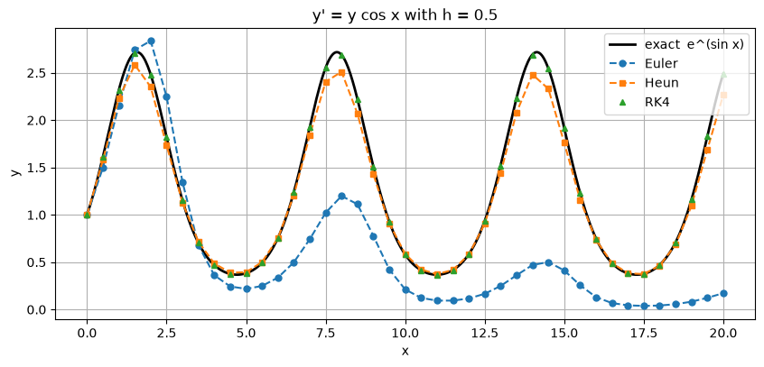
High order pays off most when the solution is smooth and the interval is long. Take

\[y' = y\cos x, \qquad y(0) = 1, \qquad \text{exact solution } y = e^{\sin x}, \qquad 0 \le x \le 20,\]

with a large step \(h = 0.5\) (only 40 steps over about three periods).

Code
w = lambda x, y: y * np.cos(x)
w_exact = lambda x: np.exp(np.sin(x))
h, n = 0.5, 40
xf = np.linspace(0, 20, 600)
plt.figure(figsize=(10, 4.2))
plt.plot(xf, w_exact(xf), "k", lw=2, label="exact  e^(sin x)")
for name, method, style in [("Euler", euler, "o--"), ("Heun", heun, "s--"), ("RK4", rk4, "^")]:
    x, y = method(w, 0, 1, h, n)
    plt.plot(x, y, style, ms=5, label=name)
    print(f"{name:6s} max |error| on [0, 20] = {np.max(np.abs(y - w_exact(x))):.2e}   ({n * {'Euler': 1, 'Heun': 2, 'RK4': 4}[name]} f evaluations)")
plt.xlabel("x"); plt.ylabel("y"); plt.title("y' = y cos x with h = 0.5"); plt.legend();
Euler  max |error| on [0, 20] = 2.32e+00   (40 f evaluations)
Heun   max |error| on [0, 20] = 2.22e-01   (80 f evaluations)
RK4    max |error| on [0, 20] = 2.20e-03   (160 f evaluations)

With only 40 steps, RK4 is visually indistinguishable from the exact solution, while Euler’s solution has drifted far from it.

3.9 Summary

  • RK4: four stages, order 4, Simpson’s rule in disguise.
  • A Butcher tableau \((A, \mathbf{b}, \mathbf{c})\) describes any Runge–Kutta method; one generic function can run them all.
  • A method has order \(p\) when its tableau satisfies all order conditions up to order \(p\). Their number grows rapidly, and beyond order 4 more stages than the order are needed.

Exercises

  1. Take one RK4 step with \(h = 0.1\) for \(y' = y\), \(y(0) = 1\). Show that the result is \(1 + h + \frac{h^2}{2} + \frac{h^3}{6} + \frac{h^4}{24}\) and compare it with \(e^{0.1}\).
  2. Show by hand that Kutta’s third-order method satisfies the four conditions for order 3.
  3. Show that for \(y' = \lambda y\) one RK4 step multiplies \(y_n\) by \(R(z) = 1 + z + \frac{z^2}{2} + \frac{z^3}{6} + \frac{z^4}{24}\) with \(z = h\lambda\). (This polynomial reappears in Section 5.)
  4. The tableau with \(c = (0, 1)\), \(a_{21} = 1\) and \(b = (1, 0)\) is consistent (\(\sum b_i = 1\)). What is its order, and why is it a poor method?

Answers

  1. \(k_1 = 1\), \(k_2 = 1 + \tfrac{h}{2}\), \(k_3 = 1 + \tfrac{h}{2} + \tfrac{h^2}{4}\), \(k_4 = 1 + h + \tfrac{h^2}{2} + \tfrac{h^3}{4}\). Substituting gives the Taylor polynomial: \(1.1051708\overline{3}\) against \(e^{0.1} = 1.1051709181\).
  2. \(\mathbf b\cdot\mathbf 1 = \tfrac16 + \tfrac23 + \tfrac16 = 1\); \(\ \mathbf b\cdot\mathbf c = \tfrac23\cdot\tfrac12 + \tfrac16 = \tfrac12\); \(\ \mathbf b\cdot\mathbf c^2 = \tfrac23\cdot\tfrac14 + \tfrac16 = \tfrac13\); \(\ A\mathbf c = (0, 0, 2\cdot\tfrac12) = (0, 0, 1)\), so \(\mathbf b\cdot A\mathbf c = \tfrac16\).
  3. Same calculation as Exercise 1 with \(\lambda y\) in place of \(y\).
  4. It is Euler’s method with a wasted second stage: \(\mathbf b\cdot\mathbf c = 0 \ne \tfrac12\), so order 1, at twice Euler’s cost.
Code
_, y = rk4(lambda x, y: y, 0, 1, 0.1, 1)
h = 0.1
print(f"1.  RK4 step = {y[1]:.10f},  Taylor polynomial = {1 + h + h**2/2 + h**3/6 + h**4/24:.10f},  e^0.1 = {np.exp(0.1):.10f}")
print(f"2.  Kutta3 order from conditions: {order_of(TABLEAUX['Kutta3'])}")
waste = {k: np.array(v, dtype=float) for k, v in dict(c=[0, 1], A=[[0, 0], [1, 0]], b=[1, 0]).items()}
print(f"4.  order from conditions: {order_of(waste)}")
1.  RK4 step = 1.1051708333,  Taylor polynomial = 1.1051708333,  e^0.1 = 1.1051709181
2.  Kutta3 order from conditions: 3
4.  order from conditions: 1